Navigation
Install the app
How to install the app on iOS
Follow along with the video below to see how to install our site as a web app on your home screen.
Note: This feature may not be available in some browsers.
More options
You are using an out of date browser. It may not display this or other websites correctly.
You should upgrade or use an alternative browser.
You should upgrade or use an alternative browser.
excel gurus
- Thread starter Bigjay73
- Start date
thebestusernamesaretaken
Well-known member
- Joined
- Feb 19, 2021
- Messages
- 449
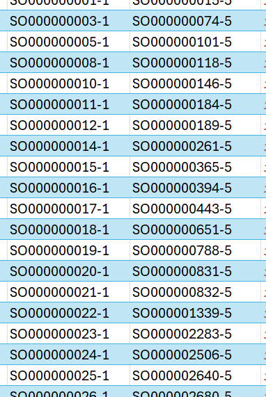
formula to find similar numbers in 2 different columns disregarding the "-#"?
That won’t work because that method won’t exclude the “-#”.
Use the formula =left([cell],11) to chop off the -# from each cell. Do this for both columns. After that the above method of conditional formatting would work. Or you could use something like =countifs([cellrange],[cell]) and it will tell you how many times that number appears in the other set.
Use the formula =left([cell],11) to chop off the -# from each cell. Do this for both columns. After that the above method of conditional formatting would work. Or you could use something like =countifs([cellrange],[cell]) and it will tell you how many times that number appears in the other set.
Bigjay73
Well-known member
Thank you!!
Johnny Bravo
Well-known member
- Joined
- Feb 15, 2022
- Messages
- 1,209
Vlookup is what I use all the time to see what data in column a is in column b.
Schaaf
Well-known member
Bullshot
Well-known member
1) insert an empty column after each existing column of your data
2) select your 1st column, then click the DATA tab, select “Text to Columns”, Select “Delimited”, click next, uncheck “TAB” and check “OTHER”, then type a dash “-“ in the box. Click next, and finish. You should now have your 11 digit string in the 1st column and the extra modifier number that you want to ignore in the second column.
3) Repeat above on your other column of original data. You will now have 4 columns with values, give then headers if you want… “Data1”, “Mod1”, “Data2”, “Mod2” for example.
4)Using the control key to
select, highlight all the cells from Data1 and from Data2 that you want to compare.
5) Click Home tab, then select “conditional formatting” then “Highlight Cells Rules” then “Duplicate Values” then OK.
DONE
*** If you later need to put your original
data strings back together, you can use the “Concatenate” function…
Similar threads
- Replies
- 13
- Views
- 547


